Introduction

From fluctuations in the stock market to the rhythmic pulse of weather patterns and even the ebb and flow of website traffic - observable changes over time are ever present. While levels of available historic data utilized to forecast future outcomes continute to rise, available time in a day stays the same. AutoML for time series forecasting can lessen the burden of these increasing demands - and we’ll show you how to deploy a production-level model in 10 minutes with Cleanlab Studio in python or using our seamless no-code platform.

Here’s the code if you’d like to follow along with details for the project and benchmarking to other methods against Cleanlab Studio AutoML - Cleanlab Studio access is required, try here for free. Book a demo for a personalized tour - no code required. You can also download the popular PJM Energy Consumption Dataset we’re using.

Problem statement

Given a dataset of time stamps and energy consumption levels, can we develop a solution that will predict energy levels for the future?

Approach

Reframing the problem from time-series to classification, and applying Cleanlab Studio AutoML to streamline and optimize a multi-step time-consuming process.

Why transform a time-series dataset into a classification dataset?

Reframing the problem leverages classification strengths, enhancing performance, flexibility, and interpretability.

1. Model Flexibility and Variety: Access a wider range of models like random forests and neural networks, capturing patterns more effectively.
2. Handling Non-Stationary Data: Focus on classifying categories rather than predicting exact values, making it easier to handle data with changing statistical properties.
3. Performance and Accuracy: Classification algorithms often provide superior performance for categorical outcomes, improving forecast accuracy.
4. Simplified Problem Framing: Discretizing continuous variables into categories simplifies the problem and makes interpretation easier.
5. Feature Engineering and Selection: Allows for tailored feature engineering, improving model performance by including lagged values, moving averages, and external variables.
6. Robustness to Outliers: Classification models are more robust to outliers, focusing on predicting categories rather than exact values.
7. Ease of Interpretation: Results are clearer and easier to communicate to stakeholders, with outputs as categories instead of numerical values.

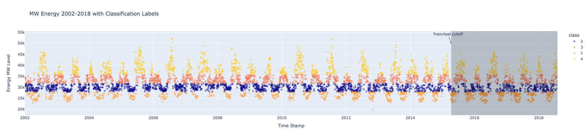
Let’s examine our dataset, which includes a datetime column and a Megawatt Energy Consumption column. We aim to forecast daily energy consumption levels into one of four quartiles: low, below average, above average, or high. Initially, we apply time-series forecasting methods like Prophet but then reframe the problem into a multiclass classification task to leverage more versatile machine learning models for superior forecasts.

Train and evaluate Prophet forecasting model

In the images above, we set the training data cutoff at 2015-04-09 and begin our test data from 2015-04-10. Using only the training data, we compute quartile thresholds for daily energy consumption to prevent data leakage from future out-of-sample data.

In order to compare to later classification models, we then forecast daily PJME energy consumption levels (in MW) for the test period and categorize these forecasts into quartiles: 1 (low), 2 (below average), 3 (above average), or 4 (high).

  python
  import numpy as np
  from prophet import Prophet
  from sklearn.metrics import accuracy_score

  # Initialize model and train it on training data
  model = Prophet()
  model.fit(train_df)

  # Create a dataframe for future predictions covering the test period
  future = model.make_future_dataframe(periods=len(test_df), freq='D')
  forecast = model.predict(future)

  # Categorize forecasted daily values into quartiles based on the thresholds
  forecast['quartile'] = pd.cut(forecast['yhat'], bins = [-np.inf] + list(quartiles) + [np.inf], labels=[1, 2, 3, 4])

  # Extract the forecasted quartiles for the test period
  forecasted_quartiles = forecast.iloc[-len(test_df):]['quartile'].astype(int)


  # Categorize actual daily values in the test set into quartiles
  test_df['quartile'] = pd.cut(test_df['y'], bins=[-np.inf] + list(quartiles) + [np.inf], labels=[1, 2, 3, 4])
  actual_test_quartiles = test_df['quartile'].astype(int)


  # Calculate the evaluation metrics
  accuracy = accuracy_score(actual_test_quartiles, forecasted_quartiles)

  # Print the evaluation metrics
  print(f'Accuracy: {accuracy:.4f}')
  >>> 0.4249

The out-of-sample accuracy is low at 43%. Not only does using only time series forecasting models limit our approach, the solution doesn’t require on-the-meter predictions. If we transform the time series data into tabular, we can quickly spin up a Cleanlab Studio AutoML solution.

Convert time series data to tabular data through featurization

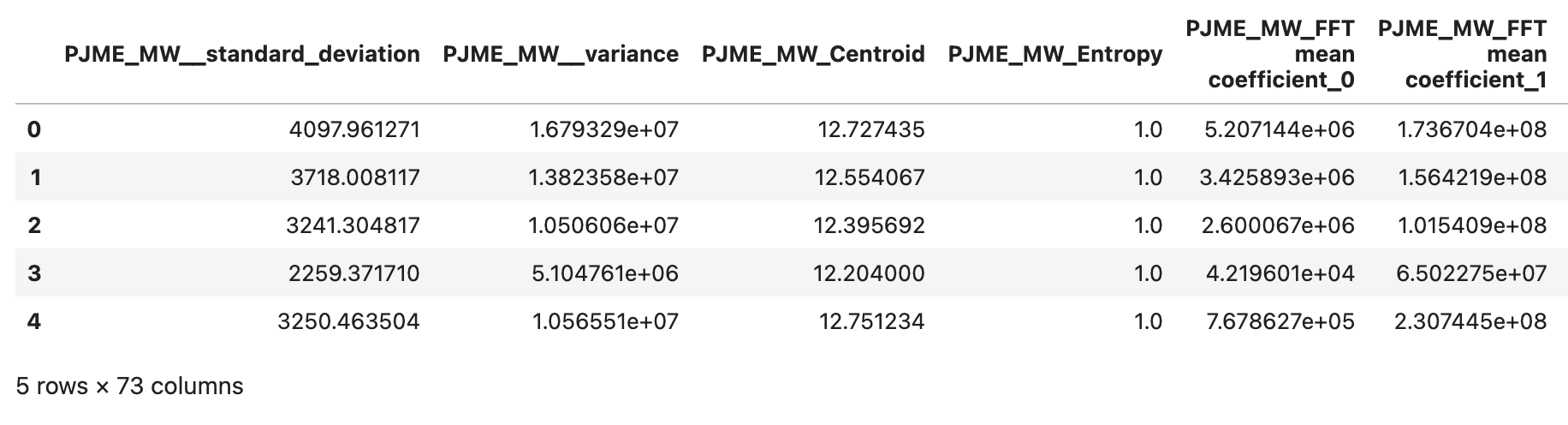
We convert the time series data into a tabular format and use libraries like sktime, tsfresh, and tsfel to extract a wide array of features. These features capture statistical, temporal, and spectral characteristics of the data, making it easier to understand how different aspects influence the target variable.

TSFreshFeatureExtractor from sktime utilizes tsfresh to automatically calculate many time series characteristics, helping us understand complex temporal dynamics. We use essential features from this extractor for our data.

tsfel provides tools to extract a rich set of features from time series data. Using a predefined config, we capture various characteristics relevant to our classification task from the energy consumption data.

python
import tsfel
from sktime.transformations.panel.tsfresh import TSFreshFeatureExtractor

# Define tsfresh feature extractor
tsfresh_trafo = TSFreshFeatureExtractor(default_fc_parameters="minimal")

# Transform the training data using the feature extractor
X_train_transformed = tsfresh_trafo.fit_transform(X_train)

# Transform the test data using the same feature extractor
X_test_transformed = tsfresh_trafo.transform(X_test)

# Retrieves a pre-defined feature configuration file to extract all available features
cfg = tsfel.get_features_by_domain()

# Function to compute tsfel features per day
def compute_features(group):
    # TSFEL expects a DataFrame with the data in columns, so we transpose the input group
    features = tsfel.time_series_features_extractor(cfg, group, fs=1, verbose=0)
    return features


# Group by the 'day' level of the index and apply the feature computation
train_features_per_day = X_train.groupby(level='Date').apply(compute_features).reset_index(drop=True)
test_features_per_day = X_test.groupby(level='Date').apply(compute_features).reset_index(drop=True)

# Combine each featurization into a set of combined features for our train/test data
train_combined_df = pd.concat([X_train_transformed, train_features_per_day], axis=1)
test_combined_df = pd.concat([X_test_transformed, test_features_per_day], axis=1)

Next, we clean our dataset by removing features with high correlation (above 0.8) to the target variable and null correlations to improve model generalizability, reduce chance of overfitting, and ensure predictions are based on meaningful data inputs.

python
# Filter out features that are highly correlated with our target variable
column_of_interest = "PJME_MW__mean"
train_corr_matrix = train_combined_df.corr()
train_corr_with_interest = train_corr_matrix[column_of_interest]
null_corrs = pd.Series(train_corr_with_interest.isnull())
false_features = null_corrs[null_corrs].index.tolist()

columns_to_exclude = list(set(train_corr_with_interest[abs(train_corr_with_interest) > 0.8].index.tolist() + false_features))
columns_to_exclude.remove(column_of_interest)

# Filtered DataFrame excluding columns with high correlation to the column of interest
X_train_transformed = train_combined_df.drop(columns=columns_to_exclude)
X_test_transformed = test_combined_df.drop(columns=columns_to_exclude)

We now have 73 features from the time series featurization libraries to predict the next day’s energy consumption level.

A quick note about avoiding data leakage

Data leakage occurs when information from outside the training dataset is used to create the model, leading to overly optimistic performance estimates and poor generalization to new, unseen data. To avoid data leakage, we applied the featurization process separately for training and test data. Additionally, we computed our discrete quartile values for energy labels using predefined quartiles for both train and test datasets.

python
# Define a function to classify each value into a quartile
def classify_into_quartile(value):
    if value < quartiles[0]:
        return 1  
    elif value < quartiles[1]:
        return 2  
    elif value < quartiles[2]:
        return 3  
    else:
        return 4  

y_train = X_train_transformed["PJME_MW__mean"].rename("daily_energy_level")
X_train_transformed.drop("PJME_MW__mean", inplace=True, axis=1)

y_test = X_test_transformed["PJME_MW__mean"].rename("daily_energy_level")
X_test_transformed.drop("PJME_MW__mean", inplace=True, axis=1)

energy_levels_train = y_train.apply(classify_into_quartile)
energy_levels_test = y_test.apply(classify_into_quartile)

Train and evaluate GradientBoostingClassifier on featurized tabular data

Using our featurized tabular dataset, we can apply any supervised ML model to predict future energy consumption levels. Here we’ll use a Gradient Boosting Classifier (GBC) model, the weapon of choice for most data scientists operating on tabular data.

Our GBC model is instantiated from the sklearn.ensemble module and configured with specific hyperparameters to optimize its performance and avoid overfitting.

from sklearn.ensemble import GradientBoostingClassifier

gbc = GradientBoostingClassifier(
    n_estimators=150,
    learning_rate=0.1,
    max_depth=4,
    min_samples_leaf=20,
    max_features='sqrt',
    subsample=0.8,
    random_state=42
)

gbc.fit(X_train_transformed, energy_levels_train)


y_pred_gbc = gbc.predict(X_test_transformed)
gbc_accuracy = accuracy_score(energy_levels_test, y_pred_gbc)
print(f'Accuracy: {gbc_accuracy:.4f}')
>>> 0.8075

With a far simpler problem of classification that still meets our needs, this accuracy of 80.75% for all classes is a great start. However, placing this model in production would still require engineering time and certainty that this model is the best for this problem.

Solution: Streamline with Cleanlab Studio AutoML

Now that we’ve seen the benefits of featurizing a time-series problem and applying powerful ML models like Gradient Boosting, the next step is choosing the best model. Experimenting with various models and tuning their hyperparameters can be time-consuming. Instead, let AutoML handle this for you.

With Cleanlab Studio, you can leverage a simple, zero-configuration AutoML solution. Just provide your tabular dataset, and the platform will automatically train multiple supervised ML models, tune their hyperparameters, and combine the best models into a single predictor. For a quick start with your own data, refer to this guide.

Here’s all the code you need to train and deploy an AutoML supervised classifier:

from cleanlab_studio import Studio

# you can find your Cleanlab Studio API key by going to app.cleanlab.ai/upload,
# clicking "Upload via Python API", and copying the API key there
API_KEY = "<insert your API key>"

# initialize studio object
studio = Studio(API_KEY)

Next load the dataset into Cleanlab Studio (more details/options can be found in this guide). This may take a while for big datasets.

dataset_id = studio.upload_dataset(dataset_path, dataset_name="training_data_pjm_daily_energy_consumption_level_for_cl_blog")
print(f"Dataset ID: {dataset_id}")

Now you can create a project using this dataset.

project_id = studio.create_project(
    dataset_id=energy_forecasting_dataset,
    project_name="ENERGY-LEVEL-FORECASTING",
    modality="tabular",
    task_type="multi-class",
    model_type="regular",
    label_column="daily_energy_level",
)

model = studio.get_model(energy_forecasting_model)
y_pred_automl = model.predict(test_data, return_pred_proba=True)

print(f"Project successfully created and training has begun! project_id: {project_id}")

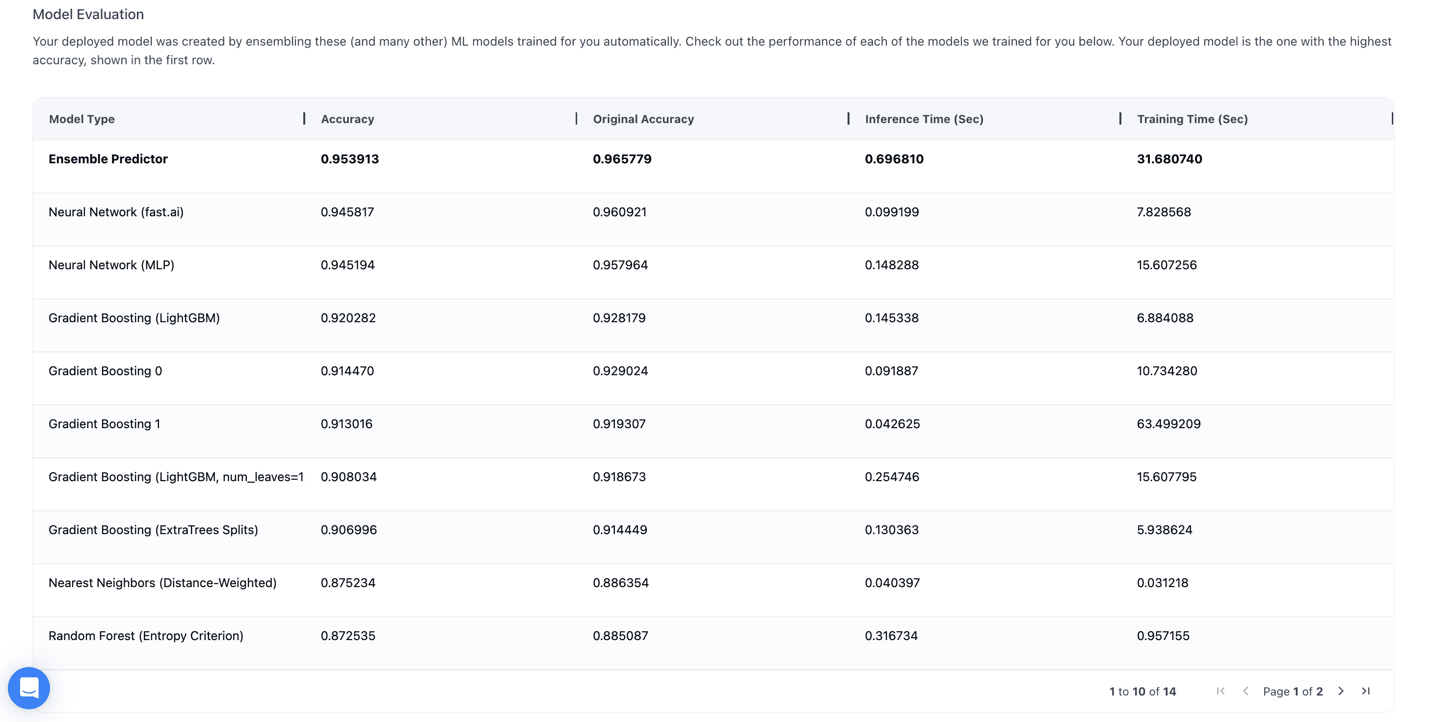
Once the below cell completes execution, your project results are ready for review!

%%time 

cleanset_id = studio.get_latest_cleanset_id(project_id)
print(f"cleanset_id: {cleanset_id}")
project_status = studio.poll_cleanset_status(cleanset_id)

Just one of the ways Cleanlab Studio simplifies the process of training a model is automatically identifying and fixing data and label issues. Once your dataset is clean, a single click with AutoML trains and deploys a reliable model suitable for production.

In the Studio interface for this project, we first used Clean Top K and Auto-Fix to address Label Issues and Ambiguous datapoints. Then, we hit Improve Results for several iterations, creating multiple Cleansets of our original data to deploy separate models.

Deploying a model for this solution is simple - click the Deploy Model button and your model will be inference-ready on new data once it’s in the ‘Deployed’ status.

After the model is deployed we check the AutoML results in our Model Details tab:

Then in our code we can fetch our model ID from the Studio Dashboard and feed it into our Python Studio object below:

# load model from Studio
# you can find your model ID in the models table on the dashboard!
model_id = "<YOUR_MODEL_ID>"
model = studio.get_model(model_id)

Using our model trained on our cleaned training data, we can run inference on our test data now to get pred_probs:

%%time

X_test_transformed["column_0"] = X_test_transformed.index
y_pred_automl_cleaned = model.predict(X_test_transformed, return_pred_proba=True)
y_pred_automl_cleaned_values = y_pred_automl_cleaned[0]

And we can now compare our out-of-sample accuracy:

cleaned_automl_accuracy = accuracy_score(energy_levels_test, y_pred_automl_cleaned_values)
print(f'Accuracy: {cleaned_automl_accuracy:.4f}')

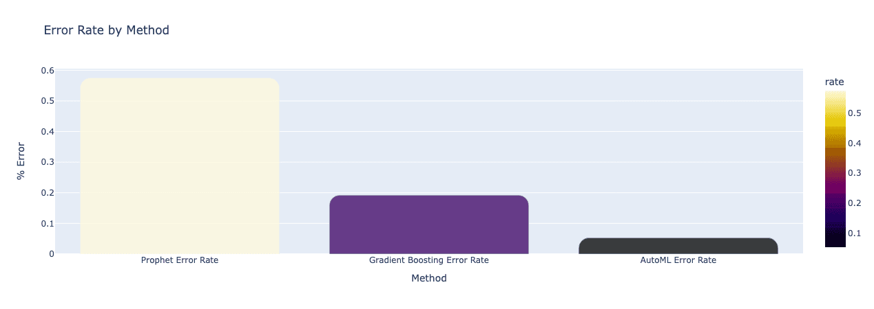
Results Recap

Conclusion

Cleanlab Studio is an advanced AutoML solution that streamlines and enhances the machine learning workflow. For time series data, converting it to a tabular format and featurizing it before deploying to Cleanlab Studio can significantly reduce development time and effort through automated feature selection, model selection, and hyperparameter tuning.

For our PJM daily energy consumption data, transforming the data into a tabular format and using Cleanlab Studio achieved a 67% reduction in prediction error compared to our baseline Prophet model. Additionally, an easy AutoML approach for multiclass classification resulted in a 72% reduction in prediction error compared to our Gradient Boosting model and an 91% reduction in prediction error compared to the Prophet model.

Using Cleanlab Studio to model a time series dataset with general supervised ML techniques can yield better results than traditional forecasting methods.

Next Steps

Transforming a time series dataset into a tabular format allows the use of standard machine learning models, enriched with diverse feature sets through feature engineering. Leveraging Automated Machine Learning (AutoML) streamlines the entire ML lifecycle, from data preparation to model deployment. Cleanlab Studio automates this process with just a few clicks, training a baseline model, correcting data issues, identifying the best model, and deploying it for predictions—significantly reducing the effort and expertise needed.

Take AutoML for a test drive today, try Cleanlab Studio for free!